Point-in-Time Weather Forecast API: Systematic Corn Futures Case Study

Executive Summary

The case study defines a simple grain futures weather-based trading algorithm focused on July.   The algorithm trades December corn futures based on the weather forecast initializations on the same day 12Z minus 00Z change in the U.S. corn production weighted 14-day precipitation forecast.  It uses thresholds statistically fit from multiple prior years of weather forecast historical data to decide long, short, or no trade as the trade

Across the backtests, performance is not broadly stable across models or holding periods. The usable signal is concentrated at the one-day horizon and is most evident for ECMWF.

The one-day ECMWF average returns are positive each year, but the gains diminish over time (means and the July sum decline materially from 2022 to 2025). GEFS and GFS at N = 1 are small and inconsistent.

Risk increases as holding periods lengthen. The best versus worst trade range widens with horizon, and longer holding periods can see downside approach or exceed upside; 2023 shows the largest swings while 2024 is the most contained.

Overall conclusion: the Point-in-Time Weather Forecast API enables objective, auditable rule design, but in these results the most defensible slice is ECMWF at N = 1, while longer holding periods and the other models do not show a stable edge.

Introduction

Grain traders frequently use weather forecasts to inform their grain futures trading, particularly during critical U.S. crop-development months such as July. This case study evaluates a systematic trading approach powered by Prescient Weather’s Point-in-Time (PiT) Weather Forecast API. The algorithm tests a December corn futures strategy across multiple Julys, using changes in the ECMWF, GEFS, and GFS models U.S. corn production-weighted 14-day accumulated precipitation forecast change in the 12Z forecast relative to the prior 00Z forecast. The trade strategy uses the forecast change to generate trade recommendations based on daily December corn futures close-to-close logarithmic returns (Equation 2) over varying lengths of day.

Logarithmic returns are defined by the following:

is the N-day close to close logarithmic return of the December corn futures contract, defined for a trading day as

The trading rules rely on objective precipitation-change thresholds derived from a seven-year history of U.S. corn precipitation forecasts and coincident futures price movements. The results of this analysis suggest two primary weather-forecast-based trades:

1. Go short December corn futures when the 00Z to 12Z change in the U.S. corn production-weighted 14-day accumulated precipitation forecast shifts drier.
2. Go long December corn futures when the 00Z to 12Z change in the U.S. corn production-weighted 14-day accumulated precipitation forecast shifts wetter.

This trading strategy is developed by quantifying the December corn futures price response over distinct three-to-eight-day periods after the precipitation forecast is issued. This is a simple price response examination designed to demonstrate PiT API trade strategy development.

The trading strategy focuses on the impact of the precipitation forecast changes on the logarithm of futures price changes over multi-day holding periods ranging from one to eight days long (Equation 2). Forward information biases are eliminated by excluding precipitation forecasts during or after the trading year under evaluation.  The following years are used to develop the trading algorithm:

• forecasts from 2017–2021 are used for the 2022 trading algorithm,
• forecasts from 2017–2022 for the 2023 algorithm,
• forecasts from 2017–2023 for the 2024 algorithm, and
• forecasts from 2017–2024 for the 2025 algorithm.

The ECMWF 12Z minus 00Z averaged (median) N-day holding-period trading returns are shown below in Table 1.

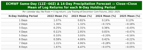
Table 1. ECMWF 12Z minus 00Z averaged (mean) N-day holding period trading returns for July trading of December corn futures in 2022 vs 2023 vs 2024 vs 2025.

Forecast vs. Futures Price Evaluation: Step-by-Step Process

The weather vs. futures quantification process is detailed below.  It’s provided to enable the reader to recreate the analysis.

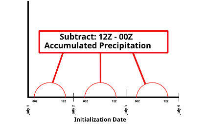
1. Use the PiT Weather Forecast API to extract ECMWF, GEFS, and GFS 00Z and 12Z U.S. corn production-weighted 14-day accumulated precipitation forecasts for all available Julys. This is achieved by retrieving the 14-day ensemble mean precipitation forecasts for each July initialization date and time. For each initialization date and time, sum the forecasted daily precipitation for each model, resulting in the accumulate precipitation forecast.

• For the 2022 trading algorithm, limit use to the July forecasts and observations from 2017–2021 (Figure 1);
• for the 2023 trading algorithm, limit use to the July forecasts and observations from 2017–2022 (Figure 2);
• for the 2024 trading algorithm, limit use to the July forecasts and observations from 2017–2023 (Figure 3);
• for the 2025 trading algorithm, use the 2017–2024 Julys (Figure 4).

2. Use the Point-in-Time Weather Forecast API to extract observed US corn production weighted precipitation climatology to compute the 14-day accumulated precipitation as a percent of normal (Equation 1a) for each 14-day forecast period. Calculate the change in the same-day 14-day precipitation forecast period change as the 12Z initialization accumulated 14-day precipitation minus the 00Z initialization accumulated 14-day precipitation from the same forecast initialization date (Equation 1c). Exclude the current trading year from the estimation set to avoid forward-information bias. See the image below as an example of this calculation and step 2.

 

3. Retrieve the July closing prices of the December 2022, December 2023, December 2024, and December 2025 corn futures contracts. Compute N-day (1–8) logarithmic returns and pair them with the daily July precipitation initialization date forecast changes by model and N-day change.

Compare the forecast changes and one of the N-day prices changes in a scatter plot.  In this case, we define the short trade (going short) threshold as the x-intercept and the long trade (going long) threshold at zero, as is defined in Equation 3.  These thresholds determine whether or not a position is taken each day of the backtest. The red lines in Figure 1 highlight the going short thresholds (x-intercept).

This trading algorithm focuses on the one to eight-day futures price close-to-close logarithmic returns which had the strongest relationships. Table 2 provides an example of this step and shows the Figure 1 data is used.

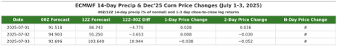
Table 2. Data example used to explain Step 3 and shows the data in that is used in Figure 1.

4. Compare the weather forecasts with the December corn futures contract closing price for July 2017 – 2021, 2017 – 2022, July 2017 – 2023, and July 2017 – 2024.
   • Compute close-to-close logarithmic returns over 1–8-day horizons for each July trading day. Figures 1–4 plot the N-day (N = 1–8) close-to-close logarithmic returns against the same-day change in the 14-day accumulated precipitation forecast, defined in Equations (1a)–(1c). The identical analysis is repeated for the GEFS and GFS models.

Equation 1.

For each forecast cycle ,

where

and

Define the forecast change of the accumulated 14-day precipitation forecast (expressed as a change in percent of normal) as

where

• is the 14-day precipitation forecast from cycle expressed as percent of normal,
• is the accumulated 14-day model precipitation forecast (ECMWF, GEFS, or GFS) from cycle ,
• is the accumulated 14-day climatological precipitation from the PiT archive,
• is the same-day change in the 14-day accumulated precipitation forecast (12Z minus 00Z) that is used as the predictor in the regression and trading algorithm.

 

5. Compute, via Equation 2a, the slope of N-day close-to-close logarithmic returns against the same day 14-day precipitation forecast change (12Z minus 00Z) for every horizon N across all weather forecast models.

Equation 2.

For each horizon , model , and trading year ,

where

• is the N-day close to close logarithmic return of the December corn futures contract, defined for a trading day as

with the settlement close on day  and the settlement close N trading days later (this matches in the R code),

• is the same day change in the 14-day accumulated precipitation forecast in percent of normal, defined in Equation 1c as
  ,
• ,
• ,
• (the trading strategy focuses on ),
• is the intercept, is the slope, and is the residual.

Ordinary Least Squares (closed form estimates). For a given and July estimation sample ,

X-intercept (short threshold). The forecast change level where the fitted line crosses zero logarithmic return is

The fitted relationships indicate that a negative change in the 14-day precipitation forecast (12Z minus 00Z) tends to be associated with a positive N-day close to close logarithmic return, while a positive change in the 14-day precipitation forecast tends to be associated with a negative N-day close to close logarithmic return over the holding period.

The algorithm sets trading thresholds from these fits. For each year (2022, 2023, 2024, or 2025), model, and N-Day horizon, the short (sell) threshold is the x intercept in Equation 2b, and the long (buy) threshold is zero. The strongest relationships typically occur for horizons , which is where the trading algorithm concentrates.

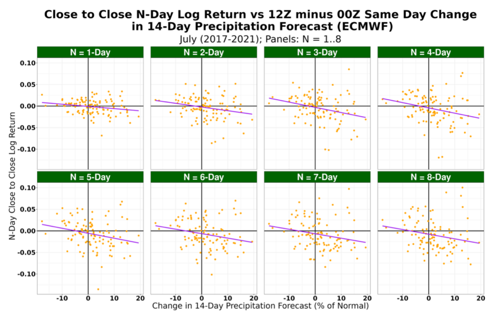
Figure 1. N-day percent December corn futures close-to-close logarithmic returns vs the change in 14-day precipitation forecast from 2017-2021. The red vertical lines highlight x-intercepts or the short trade (going short) thresholds.

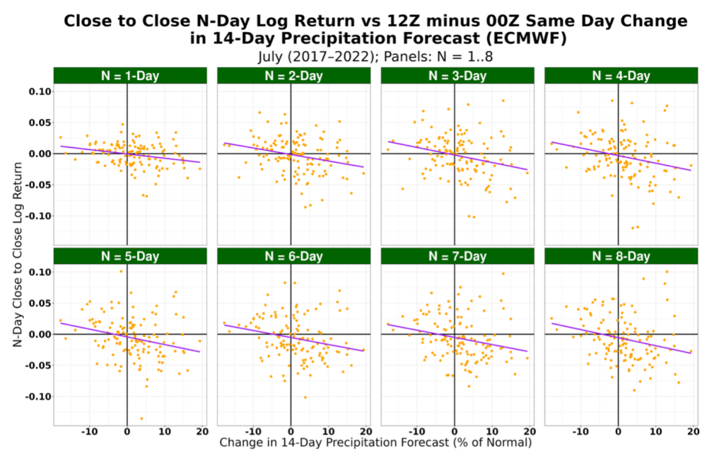
Figure 2. N-day percent December corn futures close-to-close logarithmic returns vs the change in 14-day precipitation forecast from 2017-2022.

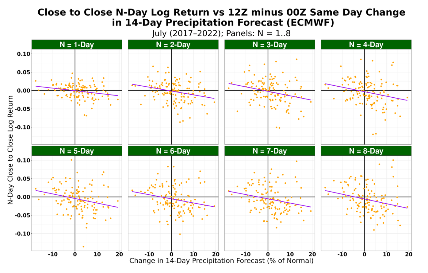
Figure 3. N-day percent December corn futures close-to-close logarithmic returns vs the change in 14-day precipitation forecast from 2017-2023.

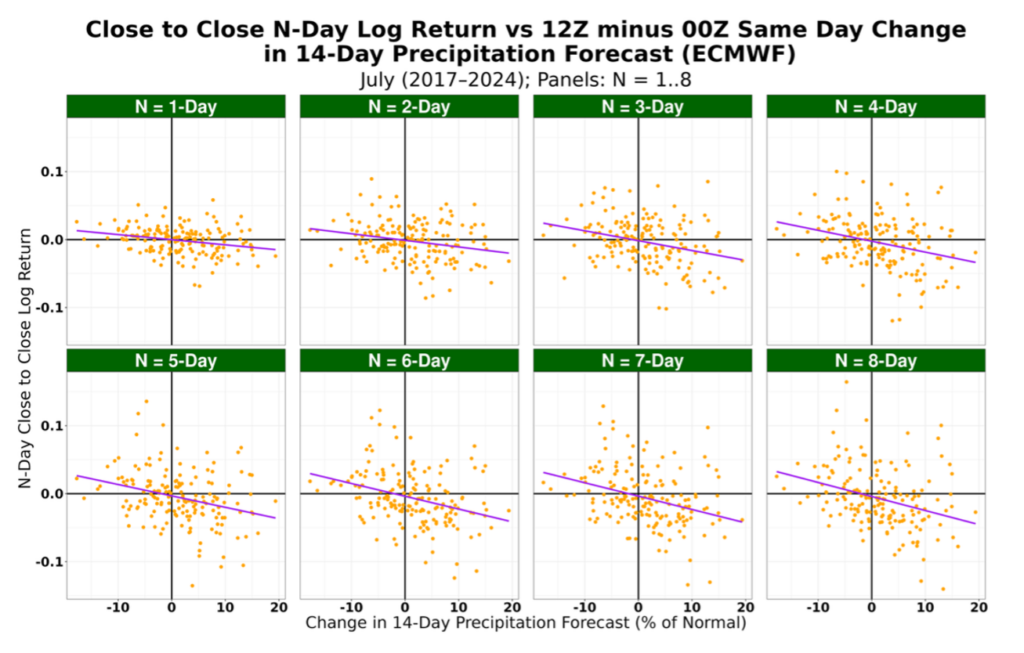
Figure 4. N-day percent December corn futures close-to-close logarithmic returns vs the change in 14-day precipitation forecast from 2017-2024.

6. Enter a trade based on the change in the 14-day precipitation forecast:
   • go short when the forecast change is greater than or equal to the short threshold,
   • go long when it is less than or equal to the long threshold, and
   • make no trade when it falls between the two thresholds (Equation 3).

Equation 3.

Let be the change in the 14 day precipitation forecast (percent of normal), and let
and (the year, model, and horizon specific x intercept from Equation 2b). Then

7. For the 12Z minus 00Z forecast change and N-day price change, evaluate returns using the thresholds: if no trade, return = 0; if long, return = price percent change; if short, return = −1 × price percent change (Equation 4). Figures 5 -7 present these results.

 

Equation 4.

Let be the N-day close-to-close logarithmic return of December corn futures.

8. For each model, compute the average (mean and median) N-Day holding period returns for July trading of December corn futures in 2022, 2023, 2024, and 2025. Table 1 summarizes these results.

Results:

Trading Algorithm Return Results for 2022, 2023, 2024, and 2025

Figures 5 through 8 display N-day (1–8) returns generated from the long/short thresholds for the ECMWF 12Z minus 00Z initialized forecast changes. July 2022 returns almost all positive outcomes across models and horizons (Figure 5). In July 2023, the returns also skew positive across models and horizons. In July 2024 (Figure 7) and July 2025 (Figure 8), returns skew slightly negative across models and horizons. These graphics summarize the rule-based outcomes for each N-day close-to-close logarithmic return by model, providing a horizon-by-horizon view of how the precipitation forecast changes driven thresholds translate into realized returns.

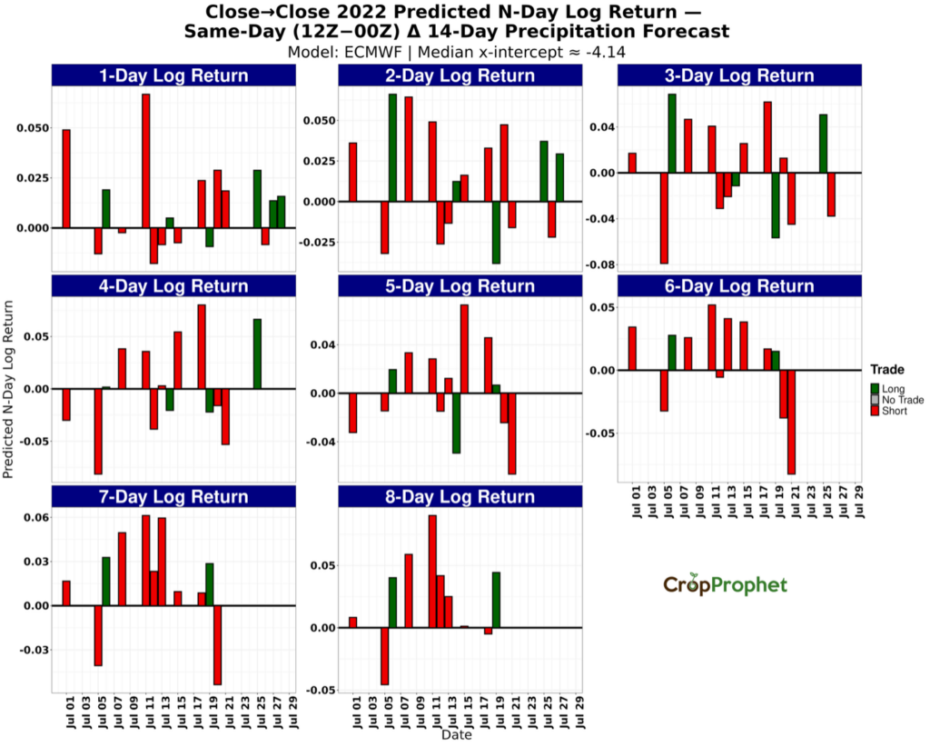
Figure 5. N-day logarithmic price returns from July 2022 precipitation forecast changes (12Z minus 00Z) based long and short trading thresholds.

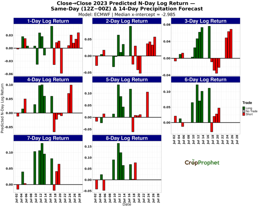
Figure 6. N-day logarithmic price returns from July 2023 precipitation forecast changes (12Z minus 00Z) based long and short trading thresholds.

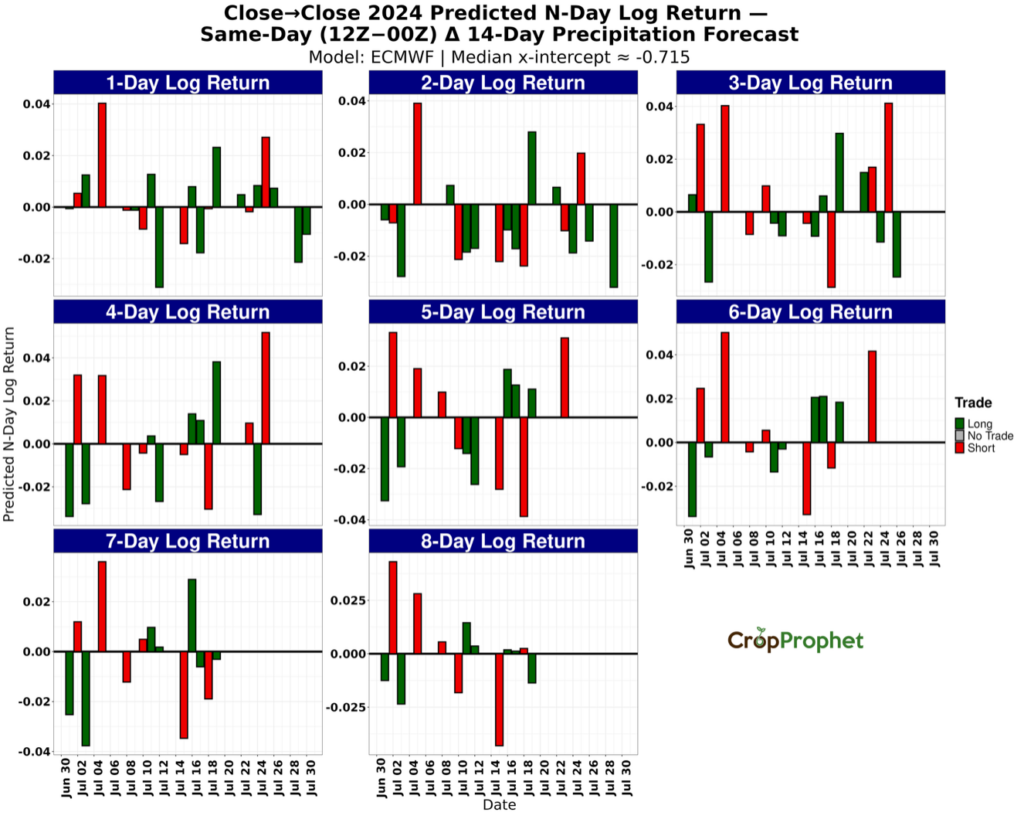
Figure 7. N-day logarithmic price returns from July 2024 precipitation forecast changes (12Z minus 00Z) based long and short trading thresholds.

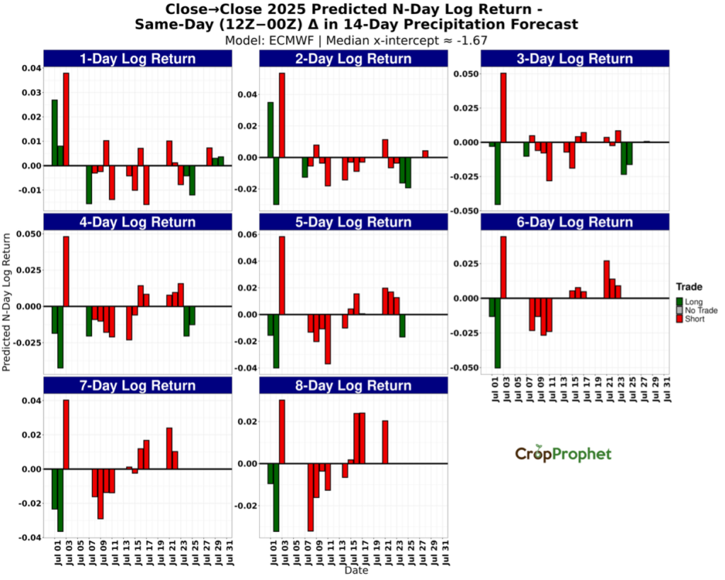
Figure 8. N-day logarithmic price returns from July 2025 precipitation forecast changes (12Z minus 00Z) based long and short trading thresholds.

Average (Mean & Median) and Sum of N-Day Holding Period Trading Returns in 2022, 2023, 2024, and 2025

To gauge performance by model at the one-day horizon, the tables show a consistent pattern: the only repeatable edge is concentrated at N = 1 and is most evident for ECMWF. For ECMWF, N = 1 average mean returns are positive in every year (about 1.07% in 2022, 0.82% in 2023, 0.19% in 2024, and 0.13% in 2025). N = 1 medians are positive in 2022–2023 (roughly 0.50% and 1.33%) and near zero to slightly negative in 2024–2025 (about −0.06% in both years). The July N = 1 sum/compounded series is positive in all years but declines over time (about 22.4% in 2022, 16.9% in 2023, 4.1% in 2024, and 2.7% in 2025). GEFS at N = 1 is small and inconsistent: means hover near zero with sign changes across years (≈ 0.03%, −0.51%, 0.37%, 0.11%), medians are ~0% throughout, and the July sum flips sign (≈ 0.7%, −9.8%, 8.0%, 2.4%). GFS at N = 1 is similarly centered near zero: means are modest and mixed (≈ −0.24%, 0.02%, 0.48%, −0.02%), medians sit at ~0% (≈ −0.03% in 2025), and the July sum alternates sign (≈ −4.4%, 0.3%, 10.6%, −0.4%). Consistent with these tables, Figures 1–4 (ECMWF scatter panels) indicate the strongest and most stable linear fit between same-day   minus 00Z changes in the 14-day precipitation forecast and the next-day price move when N = 1; the relationship weakens as N increases. In short, the defensible signal resides at N = 1 for ECMWF; GEFS and GFS do not show a durable N = 1 edge.

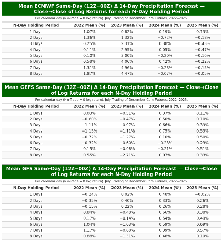
Table 3. ECMWF, GEFS, and GFS 12Z minus 00Z averaged (mean) N-day holding period trading returns for July trading of December corn futures in 2022 vs 2023 vs 2024 vs 2025.

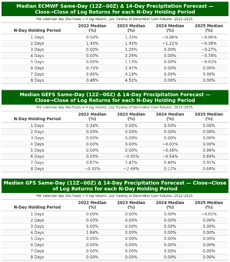
Table 4. ECMWF, GEFS, and GFS  12Z minus 00Z median N-day holding period trading returns for July trading of December corn futures in 2022 vs 2023 vs 2024 vs 2025.

Table 5. ECMWF, GEFS, and GFS 12Z minus 00Z sum of N-day holding period trading returns for July trading of December corn futures in 2022 vs 2023 vs 2024 vs 2025.

Worst Single Trades

Table 6 summarizes the largest loss observed for each N-day holding period in July trading of December corn futures (signal: same-day 12Z minus 00Z change in the 14-day precipitation forecast). The most severe outcomes occur in 2023, where worst losses deepen with horizon, from about −5.7% at N=1 to −15.2% at N=8, including large hits at N=4 (−9.5%), N=5 (−12.7%), and N=6 (−11.5%). By contrast, 2024 shows the mildest extremes across the board (roughly −3.1% at N=1–2 and −5.1% at N=8). 2025 sits between those two years, with worst losses around −2.8% at N=1 and between −3.6% and −5.0% for N=2–8. 2022 is generally moderate relative to 2023, with worst trades from about −4.8% (N=1) to −9.6% (N=5). Overall, the tail-loss profile is most contained in 2024, most pronounced in 2023 (especially at longer holding windows), and moderate in 2022–2025.

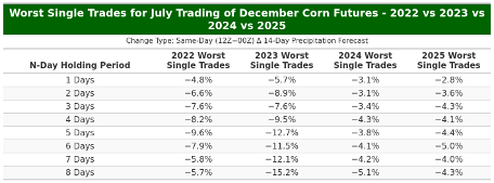
Table 6. N-day holding period worst single trades for July trading of December corn futures in 2022 vs 2023 vs 2024 vs 2025.

Best Single Trades

Table 7 reports the largest gain for each N-day holding window under the same signal. The strongest set of best trades appears in 2023, rising from about 5.2% at N=1 to 17.9% at N=8, with double-digit peaks at N=4 (10.5%), N=5 (14.5%), N=6 (13.0%), and N=7 (13.7%). The 2022 best trades are also sizable, including 10.8% at N=2 and roughly 10.5% at N=8. Best trades in 2024 are smaller and more uniform, roughly 3.7% to 5.3% across N. In 2025, best trades are mid-single-digit across horizons, from about 3.9% at N=1 to 6.1% at N=5.

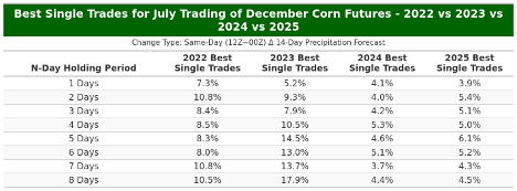
Table 7. N-day holding period best single trades for July trading of December corn futures in 2022 vs 2023 vs 2024 vs 2025.

 

The two tables above (Table 6 and Table 7) tell a consistent story about upside versus downside by year and by holding window. In 2023 the spread between the best and worst trades is widest: very large winners (up to about +17.9% at N=8) appear alongside very large losses (down to about −15.2% at N=8). In 2024 both tails are the tightest, with best trades clustered near +4–5% and worst trades around −3–5% across N, while 2025 sits between those two years and 2022 is moderate-to-large on both tails. Across horizons, N=1 shows the most favorable skew—best trades generally exceed worst trades in every year (e.g., 2022 +7.3/−4.8, 2023 +5.2/−5.7, 2024 +4.1/−3.1, 2025 +3.9/−2.8). As N lengthens, both tails expand and the downside can catch up to or surpass the upside (e.g., 2024 at N=8 best ≈ +4.4 vs worst ≈ −5.1). Taken together, the “best trade” table shows the gross opportunity available, while the “worst trade” table sets the risk floor for the same signal; comparing them suggests the one-day window offers the most attractive balance of potential gain to tail risk, whereas longer holding periods introduce materially larger swings in both directions.

Other Possible Applications:

The Point-in-Time Weather Forecast API provides crop production-weighted weather indices for the US, Argentina, Brazil, Europe, and Canada for crops you can see here.

This case study represents a single analysis; many others are possible, such as:

• US soybean-production weighted precipitation forecasts and soybean futures,
• Canadian oats-production weighted precipitation forecasts and oats futures, and
• Brazil coffee, corn, soybean, and sugar cane-production weighted precipitation forecasts and their respective futures amongst others.

As noted earlier, this case study examines a potential systematic trading strategy and how to leverage data from the Point-in-Time Weather Forecast API.  Additional analysis could normalize the December corn future prices over N-day rolling periods to minimize the day-to-day price volatility.

We expect that systematic trading applications will incorporate additional non-weather data to augment the analysis and identify stronger signals.

Conclusion:

This case study shows how Prescient Weather’s Point-in-Time Weather Forecast API can support a simple July trading rule for December corn that uses the same-day 12Z minus 00Z change in the U.S. corn production-weighted 14-day precipitation forecast and close-to-close log returns. The rule is defined as follows: fit a straight line between the forecast change and the N-day return using only prior years and identify where that line crosses zero (the fitted zero-return forecast-change level for that year, model, and horizon). Set two decision levels: zero change and the fitted zero-return level. Go short whenever the forecast change is zero or wetter; go long whenever the forecast change is at or drier than the fitted zero-return level; make no trade when the forecast change lies between those two levels or when the fitted level cannot be estimated.

Across the tests, the usable signal is concentrated at the one-day horizon and is most evident for ECMWF. At N=1 day, ECMWF shows positive average returns in each year, medians that are positive in 2022 and 2023 and near zero to slightly negative in 2024 and 2025, and July sums that remain positive but diminish over time. GEFS and GFS at N=1 are small and inconsistent.

The best-vs-worst trade tables provide the risk envelope around that signal. At N=1, the best trades exceed the worst trades in every year (for example, 2022 about +7.3 vs −4.8, 2023 about +5.2 vs −5.7, 2024 about +4.1 vs −3.1, 2025 about +3.9 vs −2.8). As the holding window lengthens, both tails widen and the downside can approach or exceed the upside (for example, 2024 at N=8 best about +4.4 vs worst about −5.1). Year-to-year, 2023 exhibits the largest swings on both tails, 2024 is the most contained, and 2025 sits between those two with 2022 generally moderate.

Overall, the API supplies the point-in-time weather history needed to design and audit objective rules. In these results, ECMWF at N=1 is the most defensible slice; longer holding periods and the other models do not present a stable edge given the observed best-to-worst trade profile.